The focus of this post is detecting the ingredients in images of food items. Such a problem falls in the realms of image classification and object detection, which have been well-studied by deep learning practitioners. One of the most popular algorithms for this is Convolutional Neural networks (CNNs). As for the datasets to choose from, the largest of the lot is Recipe1M+ from MIT. In all honestly, I would’ve loved to use this dataset for my work, but in all honesty, it is a behemoth at easily 100+ GB of data. Therefore, I decided to pick a more manageable dataset, which happened to be the Food101 dataset, at a much more manageable 4.65GB. These 101,000 come with ingredient labels and are pre-split into a train and test dataset to allow for comparisons with similar prior research. For example, researchers at the University of Barcelona have tried using deep learning models on Food101, and the paper can be read here. I’ll be using their work as a benchmark for this piece.

That’s enough of an intro. Now, to get to the interesting part. The approach! How are we going to build this neural network to help us classify and identify food images? Let me spell it out for you

Data Preprocessing

• The dataset is split into three sets- train, validation, and test sets of sizes 67.5%, 7.5%, and 25% respectively
• 227 ingredients are then transformed into a 227-size vector using MultiLabelBinarizer
• Every image is associated with this 227-ingredient vector with the value set to 1 if the ingredient is present, and 0 otherwise.

Selecting the best Neural Network

A total of 3 Neural network architecture types were utilized here. Given that the benchmark research used ResNet-50 and Inception-V3, these were replicated here. In addition, DenseNet-161 was used as it resulted in interesting results in some related work on Food101 (see here).

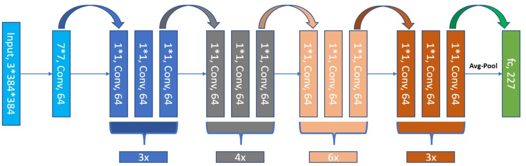
All the neural networks were pre-trained on ImageNet data (full training them would have taken ages to run). Additionally, I decided to utilize the power of transfer learning by Freezing all the network’s layers except for the last fully connected layer. In the figure above, this would be the green layer at the end of the network. I also tried unfreezing the penultimate layer, but that yield better results. Therefore, I decided to train the final layer only. Here is why I think it worked better:

• Food 101 has much fewer images than ImageNet, with 101,000 and nearly 14 million images respectively. Training the entire neural network on these 101k images can lead to overfitting, and an inability to generalize.
• To build on generalization, the pre-trained neural networks are known to be good at identifying various features/textures, and thus it is a good idea to preserve that ability, which is likely embedded in the deeper layers.
• And to build on the previous point, the final layer tends to be most responsible for classification. So training this final layer by itself tunes the network for this task while maintaining the inherent feature recognition behavior embedded in the deeper layers.

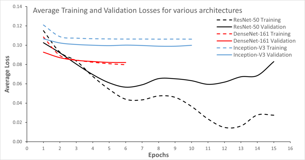
The figure above shows the loss curves for each neural network implementation. As you may be able to tell, I have implemented early stopping, which is why the loss curves terminate after being stable for a certain number of epochs.
To be honest, I was expecting DenseNet to triumph here, given its large number of parameters. There are a couple of reasons I think it didn’t beat the others:

• A dropout rate of zero– would mean that there is no regularization, leading to overfitting. Since overfitting is more pronounced for ResNet-50, I suspect this is less of a reason.
• Meaning that the more likely reason is that DesNet-161 is more sensitive to the choice of hyperparameters than the other neural networks.

It is likely that a finely-tuned set of hyperparameters could’ve resulted in better performance for DenseNet, but in the interest of time, I decided to select ResNet-50 as the model to build subsequent analysis on. Another reason to do this is that it would allow for a more direct comparison with Bolanos et al’s work.

Activation and Loss Function

From literature review, I found that when working with CNNs, the softmax activation function is typically used in the output layer. It outputs a vector consisting of a probability distribution for the potential outcomes. However, in this experiment, we would like our model to output a binary value (0 or 1) for each of the ingredients to illustrate whether the ingredient is present or not. Therefore, I decided to use the sigmoid activation function.

As for the loss, with softmax, categorical cross-entropy loss is typically used. However, given that this problem is dealing with binary classes, a binary cross-entropy loss would be a better choice.

The pretrained ResNet-50 model is subsequently trained and validated for approximately 15 epochs. A confidence threshold of 0.5 is then used to predict a positive ingredient class from the sigmoid activation function.

Model Adaptations and Tuning

The following adaptations and enhancements were used to improve ResNet-50’s performance:

Bolanos et al. were able to achieve a F1-score of (80.11%). The out-of-box ResNet-50 implementation from PyTorch, which used transfer learning described earlier with an Adam optimizer, is far from capable of doing this, therefore, the following modifications were made:

• Type 1– Unfreeze an additional layer i.e. the 3 convolutional neural networks prior to the final layer.
• Type 2– Type 1, but with a learning rate scheduler and cosine annealing used.
• Type 3- Type 2, but with the introduction of a image augmentation.

Data Augmentation can be split into two steps- the first required simple resizing of all images to 384×384 pixels, and the second was a more aggressive form of augmentation to try and reduce overfitting. Pytorch’s torch-vision transformations were key here, performing operations such as RandomResizedCrop, RandomRotation, ColorJitter, RandomHorizontalFlip, RandomVerticalFlip, RandomGrayscale, and RandomAdjustSharpness. I used this to effectively double the training dataset. Here are the loss curves:

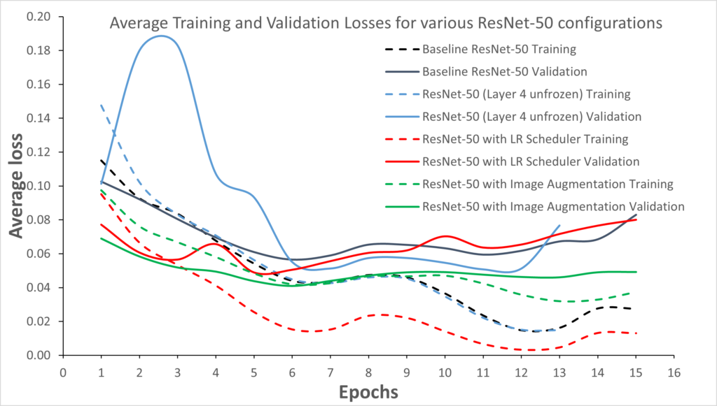
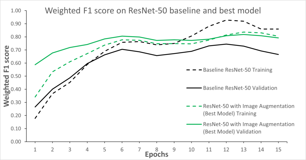
The model with the lowest validation loss is found to be the one using augmentation, which also has the lowest degree of overfitting (smallest separation between the validation and training loss curves). The F1-score curves are shown below:

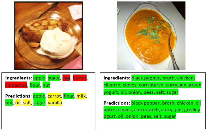
Metrics are important to look at, but it’s arguably more interesting to analyze the model’s behavior when classifying images, and how well it spots the ingredients. What was interesting is that food types that appear in different forms across dishes tend to be predicted as false negatives. This is especially true for eggs, which can appear in an omelet as a flat circular form, as poached eggs in a spherical form, as souffle in a bowl, or not even visible (e.g. in a cake). this explains why the model tends to misclassify it as shown in the images below:

In terms of comparisons with Bolanos et al’s work, the table below shows the results:

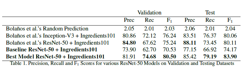
Whereas the baseline ResNet-50 model was unable to triumph Bolanos et al., the final model (with augmentations) was able to achieve a better F1-score and Recall than Bolanos. However, the Precision was not as high. This could be because a lot of augmented images helped the model to reduce false negatives thereby increasing the recall at the cost of precision.

In summary, I was able to achieve a higher F1 score than Bolanos et al. (83.9% vs 80.11%).

My GitHub repo for this package of work can be found here.