Logistic Regression using Python- A gentle introduction
I was recently invited to conduct an hour-long presentation on Logistic Regression for students. I’m fairly new to teaching, so I was quite open to the challenge and decided to embrace it. Having delivered it over 2 weeks ago, I must say that I enjoyed the experience and thought it would be worth adding to my portfolio. So without further ado, let me go deeper into it:
Background and Goal
The exercise revolved around using a smaller version of UCI’s famous Bank Marketing dataset. The original consists of 45,200 rows and 17 columns, whereas this smaller version has 15,000 rows and 5 columns. Just like with the original dataset, one of those columns serves as the target variable, which is whether the product (bank term deposit) was subscribed to (yes, or 1) or not (no, or 0).
The goal would be to build a logistic regression model that can help us predict whether or not a target variable is
Part 1: Agenda and Learning Objectives
Part 1: Agenda and Learning Objectives
Part 2: Introduction to Logistic Regression – Understand the Fundamentals
Part 3: Problem Set-up and Exploratory Data Analysis – Understand the Data
Part 4: Vanilla Implementation of Logistic Regression – Build a baseline
Part 5: Model Validation (Cross-Validation and its Importance)
Part 6: Application of Feature Engineering (e.g. one-hot encoding) – Improve model performance
Part 7: Fine-tuning – Improve model performance
Part 8: Additional Resources and Further Reading
Part 2: Introduction to Logistic Regression
Linear Regression returns continuous values, but what if we want to use the data to return binary classes (e.g. Yes or No)? Logistic Regression can help here. Instead of Maximizing R^2, Logistic Regression transforms the output of the linear function between 0 and 1 (i.e. a binary classification) using a sigmoid function and maximizes likelihood.
Part 3: Problem Set-up and EDA
The next step is to import all the libraries required. The most notable library imported is sklearn for
import numpy as np                                      # For mathematical calculations
import pandas as pd                                     # For dataset creation and manipulation

import matplotlib.pyplot as plt                         # For data visualization
import seaborn as sns                                   # For data visualization

# Machine Learning Packages
from sklearn.model_selection import train_test_split
from sklearn.linear_model import LogisticRegression
from sklearn.preprocessing import LabelEncoder

from sklearn.metrics import accuracy_score, confusion_matrix, f1_score

from sklearn.preprocessing import StandardScaler

from sklearn.model_selection import cross_validate

## Show me how to run a cross-validation grid search on the model
from sklearn.model_selection import GridSearchCV
from sklearn.metrics import make_scorer
import scipy.stats as stats
Then, we can create a dataframe from the csv file in question:
## Read the CSV file to create bank_df from bank_small.csv, and show its shape and first 5 rows
bank_df = pd.read_csv('bank_small.csv')
print(bank_df.shape)
bank_df.head()

Output:
"""
        loan	duration	poutcome	job	y
0	no	1042	         unknown	admin.	yes
1	no	1467	         unknown	admin.	yes
2	no	1389	         unknown	technician	yes
3	no	579	         unknown	services	yes
4	no	673	         unknown	admin.	yes
"""
Descriptions for each of the features are shown below:
● loan: if the client currently holds a loan
● duration: last contact duration in seconds
● poutcome: outcome of the previous marketing campaign
● job: the occupation of the client
● y: whether the client signed up for the new term deposit
Let’s also look at the type(s) of data we are dealing with here:
## Let's look at the type of data we are dealing with
bank_df.dtypes
Output:
"""
loan object
duration int64
poutcome object
job object
y object
dtype: object
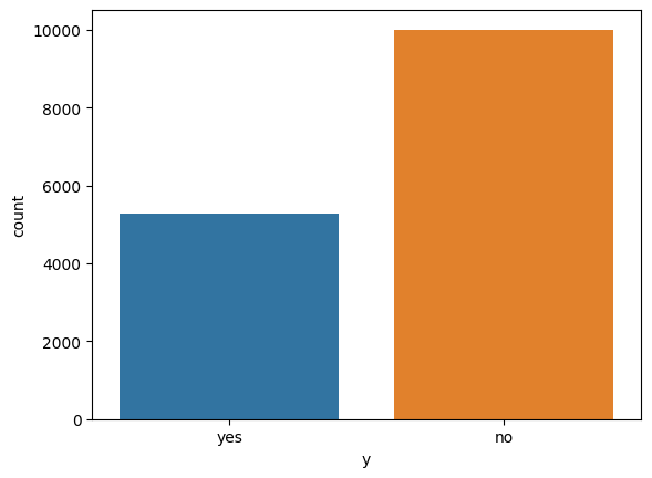
"""Additionally, a plot of the counts of the target variable is shown below, which shows that the target variable is slightly imbalanced in favour of no new term deposits.
Part 4: Vanilla (Baseline) Logistic Regression Model
It’s generally a good idea to build a baseline model that can be compared to all our subsequent models- in an attempt to determine the effect of our enhancements.
So to begin with, we can create a copy of the original banking dataset, and call this “bank_df_copy”
bank_df_copy = bank_df.copy(deep=True)Logistic Regression cannot run with text/string data. Therefore, we have to change the data numbers using Python’s “LabelEncoder”. We apply it to all the fields that are categorized as an “object”:
le = LabelEncoder()
bank_df_copy['loan'] = le.fit_transform(bank_df_copy['loan'])
bank_df_copy['poutcome'] = le.fit_transform(bank_df_copy['poutcome'])
bank_df_copy['job'] = le.fit_transform(bank_df_copy['job'])
bank_df_copy['y'] = le.fit_transform(bank_df_copy['y'])
bank_df_copy.head()
Output:
"""
loan duration poutcome job y
0 0 1042 3 0 1
1 0 1467 3 0 1
2 0 1389 3 9 1
3 0 579 3 7 1
4 0 673 3 0 1
"""Notice how the “job” column now has numbers assigned as opposed to words. This will now make it work with machine learning models using the scikit learn package.
Next, we need to split the datasets based on the features we want to train the machine learning model on, and the the labels we want to learn. This would be “X” and “y” respectively
X = bank_df_copy.drop('y', axis=1)
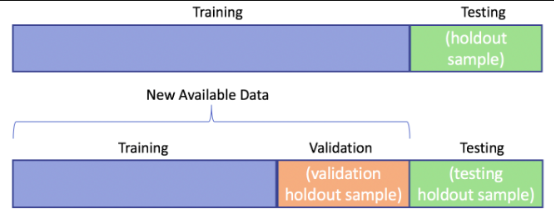
y = bank_df_copy.yAs the next figure shows, the original data needs to be split into a train and a test dataset. In machine learning, it is best practice to train our model on a training dataset, and hold-out a test dataset to assess out model’s performance on unseen data. This helps us determine how well out model performs with unseen data, and if it does perform well on unseen data, then we can conclude that our model generalizes well.
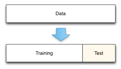
In this example, we choose a 80:20 data split for our dataset (training:test). (Note the inclusion of “random_state”. This will be used multiple times, and it is important because it allows us to repeat the exact same data split or iteration if we were to call the method/function again).
X_train, X_test, y_train, y_test = train_test_split(X, y, test_size=0.2, random_state=14)Notice how we have now split “X” and “y” into training and testing sets.
Next, we can create our Vanilla Logistic Regression model, and fit it to the training data.
logmodel = LogisticRegression(max_iter=1000, random_state=14)
logmodel.fit(X_train, y_train)
Now we have a trained Logistic Regression model, and we can use it to predict labels from our test dataset:
y_pred = logmodel.predict(X_test)As shown below, calling the prediction function outputs an array of binary values as predictions:
y_pred

Output:
"""
array([1, 0, 0, ..., 0, 1, 0])
"""
Next, we can call scikit-learn’s “accuracy_score” function to quantify the number of values that our model guessed correctly:
accuracy_score(y_pred, y_test)

Output:
"""
0.7678221059516024
"""
Our Model has 76.8% Accuracy!
However, we have to take something into consideration- Accuracy is only concerned about the values the model guessed correctly. This may sound like what we want, but it is flawed.
Take this example- if we had an array of only zeroes, our accuracy would be around 66%. By that logic, our Vanilla model may be quite poor at predicting 1’s, getting most of its accuracy from the larger number of 0’s it has.
Therefore, we can use a metric known as the F1-score. F1-score is better suited for datasets with such an imbalance. It takes the precision and recall into consideration for calculations, finding their harmonic mean.
f1_score(y_pred, y_test)

Output:
"""
0.5928899082568807
"""
As we can see, our model has a F1-score of 59.3%.
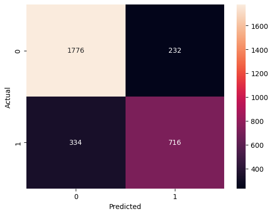
Additionally, it is useful to analyze the confusion matrix of our model. This helps us undesrtand how effective our model is at correctly predicting labels, and how many false negatices and/or false positives are produced.
def cm_plot(y_test,predictions_test):
    cm = confusion_matrix(y_test,predictions_test)
    sns.heatmap(cm, annot=True, fmt='d')
    plt.ylabel('Actual')
    plt.xlabel('Predicted')
    plt.show()
cm_plot(y_test,y_pred)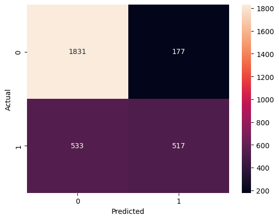
As the confusion matrix shows, the model predicts a dispropotionately larger number of false negatives (where model predicts negative, and the actual is positive) when compared to the number of false positives. This means that the vanilla model has a slight preference to predict that the client won’t sign up for a new term deposit, whereas in reality, the client does sign up.
Another interesting aspect to analyze is the frsture importance graph, as shown below:
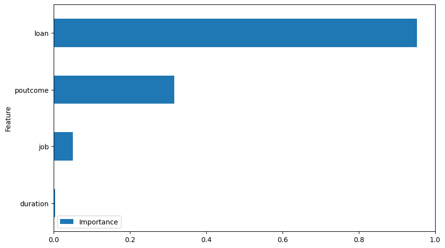
This shows that the model considers the “loan” feature as the most imporant one in deciding whether of not the client signs up for a new term deposit.
Part 5: Model Validation (Cross-Validation)
Another commandment in Machine Learning: Do not use your test dataset to tune your model.
Instead, we should use a validation dataset instead. Therefore, the previous train-test split now becomes a train-validation-test split, as shown in the diagram below:
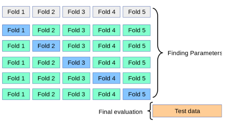
However, rather than relying on a single portion of the data to act as a validation set, it is common to use an approach called Cross-Validation instead.
What is Cross-Validation? It involves splitting the data into folds (5 in our case), and using 1 of those folds as a validation set, whilst the others remain as a training set. Then, we keep rotating the validation set until all the categories have been used as a validation set. The Diagram below shows this, where the Folds shown in blue are essentially the validation sets across 5 iterations (the number of folds and iterations are equal). Notice how the test data set is held-out till the end for final evaluation.
The code to implement Logistic Regression with cross-validation is shown below. (Notice how we are specifying the “F1” scoring function, rather than the
logmodel = LogisticRegression(random_state=14, max_iter=1000)
results = cross_validate(logmodel, X_train, y_train, cv=5, scoring='f1')
We can see out results from our validation set by look up the “test_score” key in the results dictionary:
results['test_score']
Output:
"""
array([0.58487874, 0.57225018, 0.55514974, 0.58158996, 0.58916968])
"""
The average score across all folds is:
np.mean(results['test_score'])
Output:
"""
0.5766076603930993
"""
Notice how the f1-score is less than what we calculated at the end of Part 4. This is because cross-validation is much better at showing us how well our model generalizes. Right now, it can certainly do better. Let’s start making some progress in that direction!
Part 6: Application of Feature Engineering
To quote the GOAT himself:
“Applied machine learning is basically feature engineering”. — Andrew Ng
Introducing one-hot encoding
There’s a drawback with Label Encoding- it tends to add order and magnitude to the data when the data has neither. One-hot encoding fixes this by insteading cretina new column for every unique value in the the categorical column in question.
We will apply it for all caterogical column with more than 2 unique values
for column in bank_df.columns:
    if bank_df[column].dtype == type(object):
        print(column, ": ",  bank_df[column].nunique())
Output:
"""
loan :  2
poutcome :  4
job :  12
y :  2
"""
As the code above shows, “poutcome” and “job” have more than 2 unique variables, therefore, we will use them for one-hot encoding. First, we stick to label encoding for the rest:
bank_df_copy = bank_df.copy(deep=True)

le = LabelEncoder()
bank_df_copy['y'] = le.fit_transform(bank_df['y'])
bank_df_copy['loan'] = le.fit_transform(bank_df['loan'])
Then, one-hot encoding is applied to “outcome” and “job” using the “get_dummies” method:
bank_df_copy = pd.get_dummies(bank_df_copy, columns=['poutcome', 'job'])Now we can look at the new columns produced:
bank_df_copy.columns

Output:
"""
Index(['loan', 'duration', 'y', 'poutcome_failure', 'poutcome_other',
       'poutcome_success', 'poutcome_unknown', 'job_admin.', 'job_blue-collar',
       'job_entrepreneur', 'job_housemaid', 'job_management', 'job_retired',
       'job_self-employed', 'job_services', 'job_student', 'job_technician',
       'job_unemployed', 'job_unknown'],
      dtype='object')
"""
Notice how “poutcome” and “job” have new columns for each unique variable.
Now, we can run our Logistic Regression model again, with the cross-validation splits like last time, and average score we get across the 5 folds:
X = bank_df_copy.drop('y', axis=1)
y = bank_df_copy['y']
X_train, X_test, y_train, y_test = train_test_split(X, y, test_size=0.20, random_state=14)

logmodel = LogisticRegression(random_state=14, max_iter=1000)
scores = cross_validate(logmodel, X_train, y_train, scoring='f1', cv=5, return_estimator=True)
scores['test_score']
np.mean(scores['test_score'])

Output:
"""
0.6720125250554365
"""
WHOA! That’s a sharp increase in the F1-score. This shows us how label encoding was leading logistic regression down the wrong path. Onehot encoding helped fix quite a bit.
Let’s have a look a the feature importance plot now:
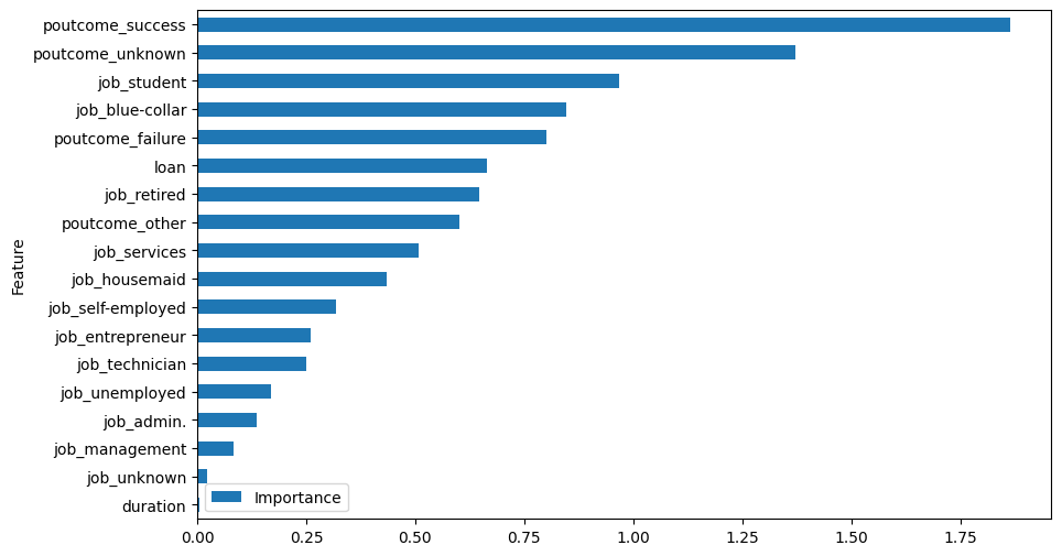
As we can see, the outcome of the previous marketing campaign is quite important. Additonally, students and blue collar individuals are most important for prediction.
Next, we can use a correlation heatmap to determine which of these features are most correlated to each other and to the target:
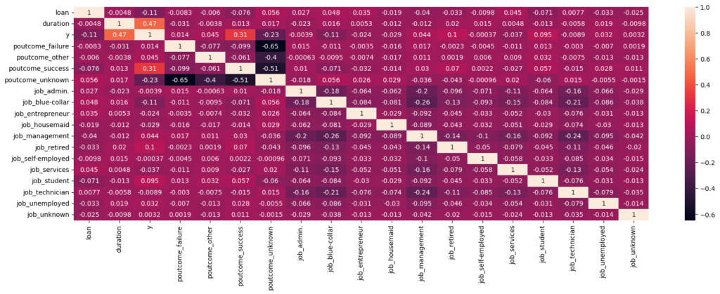
Here, we can see that the call duration and outcome of the last campaign have the largest positive correlation with the target, whereas the largest negative contribution comes when the outcome of the previous campaign is unknown.
Let’s not jump to conclusions yet though. We still have quite a bit of work in the form of enhancements that we need to do before we can even make a single conclusion.
Introducing Scaling
If we look at the duration column, it is completely out of scale relative to the rest of the columns:
X.head()

Output:
"""
	loan	duration	poutcome_failure	poutcome_other
0	0	1042	        0	                0
1	0	1467	        0	                0
2	0	1389	        0	                0
3	0	579	        0	                0
4	0	673	        0	                0
"""
We can apply something called “StandardScaler()” to address this. Standard scaler works on each column by calcualting its mean and standard devaiton, and then subtracting the value by the mean and dividing it by the standard deviation.
It is important to only fit it on the training dataset rather than the entire dataset. This makes sure that there is no data leakage, where the data from the test set influences the training dataset (because we want the model to generalize well to unseen data).
scaler = StandardScaler()
X = scaler.fit_transform(X)
Then, our training data looks like this:
X

Output:
"""
array([[-0.41551075,  2.20667423, -0.35275943, ..., -0.44181458,
        -0.17769867, -0.07823063],
       [-0.41551075,  3.52548793, -0.35275943, ..., -0.44181458,
        -0.17769867, -0.07823063],
       [-0.41551075,  3.28344683, -0.35275943, ...,  2.26339293,
        -0.17769867, -0.07823063],
       ...,
       [-0.41551075,  0.85993272, -0.35275943, ..., -0.44181458,
        -0.17769867, -0.07823063],
       [-0.41551075, -0.71643754, -0.35275943, ..., -0.44181458,
        -0.17769867, -0.07823063],
       [-0.41551075, -0.76919009, -0.35275943, ..., -0.44181458,
        -0.17769867, -0.07823063]])
"""
Now, we can convert the training set back to a dataframe using our previously stored columns:
X = pd.DataFrame(X, columns=X_columns)Now, let’s build out logistic regression again with this change:
X_train, X_test, y_train, y_test = train_test_split(X, y, test_size=0.20, random_state=14)

logmodel = LogisticRegression(random_state=14, max_iter=1000)
scores = cross_validate(logmodel, X_train, y_train, scoring='f1', cv=5, return_estimator=True)
scores['test_score']
np.mean(scores['test_score'])

Output:
"""
0.6733527326519975
"""
We git a very slight improvement. However, let’s not stop there. Let’s have a look at the Feature importance plot:
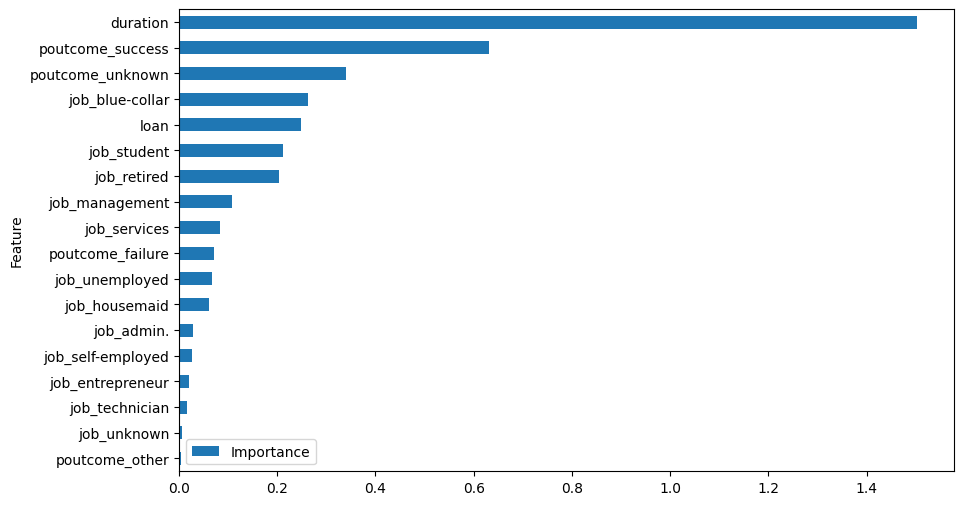
We can now see that duration has gone from the least important to the most important feature!
Fixing Extreme Skewness
Let’s look at the histogram plot of the “duration” feature:
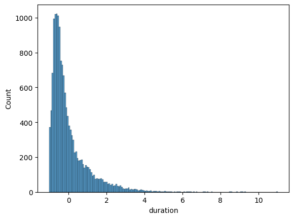
As we can see, it is extremely positively skewed. We can correct this using the yeo_johnson correction.
X['duration'], _ = stats.yeojohnson(X['duration'])sns.histplot(X.duration)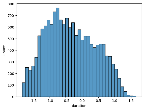
Now, we can see that the skewness has been largely rectified.
Now, let’s build out logistic regression again with this change:
X_train, X_test, y_train, y_test = train_test_split(X, y, test_size=0.20, random_state=14)

logmodel = LogisticRegression(random_state=14, max_iter=1000)
scores = cross_validate(logmodel, X_train, y_train, scoring='f1', cv=5, return_estimator=True)
scores['test_score']
np.mean(scores['test_score'])

Output:
"""
0.7004279193726474
"""
We get another enhancement over the previous answer. Let’s take this a step furhter by fine-tuning our logistic regression model using a Grid Search:
Part 7: Fine-tuning Logistic Regression using Grid Search
Grid search allows us to specify numerous parameters for tuning the model, and test each combination. The various parameters are shown below, which allows for a total of 192 combinations to be attempted.
logmodel = LogisticRegression(random_state=14, max_iter=1000)

parameters = {'C': [0.001, 0.01, 0.1, 0.5, 1, 5, 10, 25],
                'penalty': ['elasticnet', 'l1', 'l2', None], 'solver': ['lbfgs','newton-cg'],
                'tol': [1e-5 , 1e-4,  1e-3]}
Then, we fit call the Grid Search function, whilst maintaining cross-validation:
grid_obj = GridSearchCV(logmodel, parameters, scoring=make_scorer(f1_score), cv=5)
grid_fit = grid_obj.fit(X_train, y_train)
Then, we can determine our best model:
best_model = grid_fit.best_estimator_
best_model

Output:
"""
LogisticRegression(C=0.5, max_iter=1000, random_state=14, tol=1e-05)
"""
We can now look at the mean validation score:
scores = cross_validate(best_model, X_train, y_train, scoring='f1', cv=5, return_estimator=True)
scores['test_score']
np.mean(scores['test_score'])

Output:
"""
0.7005999904831042
"""
The improvement is very minimal. We can now try to assess the test score as well, by running a predicting using the tet dataset:
y_pred = best_model.predict(X_test)
f1_score(y_test, y_pred)

Output:
"""
0.7167167167167167
"""
In summary, our improvements have led to an approximate increase of 12% over the baseline model (from 59.3% to 71.7%).
If we look at the confusion amtrix below, we can see fewer false positives now (compared to the baseline model).
This is one way of doing it, and highlighting the basics of the machine learning process. Further enhancements can be made using other ML models, such as XGBoost or LightGBM. But again, this is a good start to get a general idea!